The Future Makes Fools of Us All

There is a principle from extreme programming that I quite like, “you ain’t gonna need it” (YAGNI). Here’s a post which does a good job introducing the idea. Basically, we should only implement the features we actually need, not the ones we think we might need in future. But why should we follow the YAGNI principle?

Well, in my experience, there are five good reasons.

Firstly, try as we might, we can’t see into the future. We are likely to get the requirements for this future feature wrong, because they aren’t really requirements yet. Also, we will probably operate with all kinds of assumptions that will get invalidated by the time we really need this new feature. We won’t know what we need to implement, because we don’t need to implement it yet!

Secondly, as technically minded people, we enjoy writing code and solving complex technical problems. So, we have a bias towards over-engineering. There is a good chance, we’re not actually planning ahead for future requirements, but are really just doing some fun coding. So we should always check that impulse, and make sure that we are building something that will add value right now, rather than following a fun diversion.

Thirdly, all code has bugs in it, so the more features we add, the more bugs we add. And we want as few bugs in our code base as possible. Which means we write as few features as possible. In particular, a pre-emptive feature may contain bugs itself, but it is also likely to introduce bugs in existing code paths!

Fourthly extra features mean extra complexity. This makes our code harder to monitor, support and maintain. But worst of all, it makes it harder to extend. When new requirements do arise, it will actually be harder to implement them because of the extra complexity we baked in at the start. Often times we mistake complexity for extensibility. To me, code is extensible when adding new features is quick and easy. This means that complexity is the enemy of extensibility.

Fifthly, there is always a trade off with features we need right now! Every team I have been on has had a lengthy backlog of productive work that any one of us could have taken on at any time. Rather than trying to solve a problem before it arises, why not solve a problem that already exists. Don’t sacrifice what we need right now, for what we may need in the future. Moreover, we always underestimate how much work it will take to implement some new feature, which is likely to make the trade off even worse.

So, next time, when we are tempted to add some functionality to our code, we should ask, do we really need this right now? And, rather than guessing how our code will be used in the future, admit that we don’t, and can’t know how it will be used!

Regression VIII – Looking to the Past for Inspiration

Sometimes, time series data will have certain amount of inertia. This is when the values tend to stick around whatever value they currently are at. This is a slightly weird concept, so let’s generate some toy data that illustrates it.

import numpy as np
X = np.arange(0, 1, 0.001)

Y = [0]

for in it in range(1, 1000):
    Y.append(Y[i - 1] + np.random.normal(0, 0.05))

We have created two arrays. The first, X, which is just an evenly spaced range of 1000 points from 0 to 1. The second, Y, is defined iteratively, it starts and zero and then each consecutive value is the previous value plus a draw from a random normal with mean 0 and standard deviation 0.05.

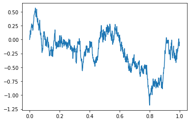
When we plot Y against X it looks like this,

We can see, that rather than varying randomly around 0, this time series will wander occasionally to a certain level and then stay near there.

So, how do we model this kind of behaviour? With a lag feature. We can define a lag feature based on Y by

lagging_predictor = [0] + Y[:-1]

For each index, this new feature will have the same value as the previous value of Y. We’ve also filled in the first value with 0.

Now let’s try some Linear Regression.

from sklearn.linear_model import LinearRegression
lagging_model = LinearRegression().fit(np.array(lagging_predictor).reshape(-1,1), Y)

When we look at the coefficients of this, we get an slope of 0.99 and an intercept of 0.003.

So our lagging model always predicts 0.003 plus 0.99 times the last value of Y. Which is a pretty good prediction! We can build more complex lagging features, but remember that linear combinations of features are taken care of by the fitting in ordinary least squares, so we don’t need to try those features ourselves.

Regression VII – New Harmonies

It is common enough when looking at time series, to see a cyclic pattern. The values in our series will oscillate predictably. This may be driven by an underlying effect based on the time of day, or the day of the week, or even the day of the year. We can model this with a little feature engineering.

What we are talking about is a wave. Any wave can be modelled as a sine function. Suppose we have a time variable t that is normalised to have values between \(0\) and \(1\), then an arbitrary wave will be of the form

\[ A\sin(o + tf2\pi) \]

where

  1. A is the amplitude of the wave, that is, how high and low each crest and trough are
  2. f is the frequency, that is, how many times the wave repeats for a single unit of time
  3. o is the offset, how much the wave is shifted forwards

Now, these terms are quite non-linear, so they will by hard to model. However, we can do a little trigonometry. Thanks to the identity

\[ \sin(\alpha + \beta) = \sin(\alpha)\cos(\beta) + \cos(\alpha)\sin(\beta) \]

we can rewrite the wave function as

\[ A\sin(o + tf2\pi) = A\sin(o)\cos(tf2\pi) + A\cos(o)\sin(tf2\pi) \]

We can then define \(B = A\sin(o)\) and \(C = A\cos(o)\), and then write any wave in the form

\[ B\cos(tf2\pi) + C \sin(tf2\pi) \]

Now the only nonlinear term is the frequency of the oscillations.

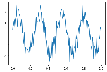
Let's look at an example, suppose we have a time series that looks like,

By eyeballing it, we can see a seasonal effect which repeats four times. So let's try some linear regression against the features \(\sin(x*4*2*\pi)\) and \(\cos(x*4*2*\pi)\).

import numpy as np
from sklearn.linear_model import LinearRegression
X, Y = # wherever our data comes from
sin_feature = np.sin(X*4*np.pi)
cos_feature = np.cos(X*4*np.pi)

harmonic_model = LinearRegression().fit([[s,c] for s,c in zip(sin_feature, cos_feature)], Y)

Now, I ran this regression myself, and the coefficents I got where, 1.69 and 0.38. So, we have

\[ A\sin(o) = 1.69, A\cos(o) = 0.38 \]

Which means our model's offset is

\[ o = \tan^{-1}(0.38/1.69) = 0.22 \]

and our amplitude is

\[ A = 1.69 /\cos(0.22) = 1.73 \]

This is pretty good, as I generated the above data with an amplitude of 1.8 and an offset of 0.2 via

import numpy as np
X = np.arange(0, 1, 0.002)
Y = 1.8*np.sin(0.2 + X*4*2*np.pi)

We won't always have such an obvious cyclical pattern where we can spot the frequency by eye. We'll be looking at how to determine the appropriate frequency in these cases in a future post.

Regression VI – Polynomial Features

It’s time to talk about feature engineering. Using just the tools of linear regression, we can greatly increase the complexity of our models by creating features from our underlying data. A feature is a new predictor that we create by applying some function to our existing set of predictors. We can think of it as manipulating the data to dig out underlying patterns.

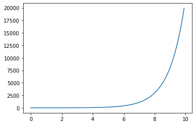
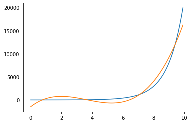
The best example are polynomial features. Suppose we have a single predictor X which is spaced evenly between 0 and 10, and a response Y. Say we plot Y against X and it looks like this

Lets try and do a simple linear regression against Y.

import numpy as np
from sklearn.linear_model import LinearRegression
from matplotlib import pyplot as plt

linear_model = LinearRegression().fit([[x] for x in X],Y)
linear_predictions = linear_model.predict([[x] for x in X])
plt.plot(X,Y)
plt.plot(X, linear_predictions)
plt.show()

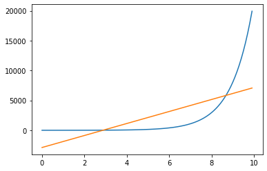
This will create something like this

Not very good at all. So, let’s try adding a new feature. We will define this feature as the square of X, like so

square_model = LinearRegression().fit([[x, x**2] for x in X], Y)
square_predictions = square_model.predict([[x, x**2]])
plt.plot(X,Y)
plt.plot(X, square_predictions)
plt.show()

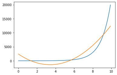
This will give you something that looks a bit better

Although our regression is still linear, now we are fitting the closest quadratic rather than the closest straight line. This is also called polynomial regression. But I think it makes more sense to think of it as a form of feature engineering.

Now, let’s add another feature, the cube of X.

cubic_model = LinearRegression().fit([[x, x**2, x**3] for x in X], Y)
cubic_predictions = cubic_model.predict([[x, x**2, x**3]])
plt.plot(X,Y)
plt.plot(X, cubic_predictions)
plt.show()

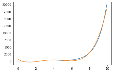
Now we’re getting there. If we add the fourth powers of X as a feature, we will get an even better looking fit

We are not just limited to polynomial features, as we shall see. However we shouldn’t bother with linear features, as any linear term is already captured in the regression itself. When we fit, we already find the best possible linear combination of the predictors . So our features need to be non-linear in our existing predictors. A big part of building and fitting models is finding useful features in our data like this.

Regression V – Why does OLS make me so blue?

When we derived our formula for the coefficients of regression, we minimised the sum of the squares of the difference between our predicted values for \(Y\) and the true values of \(Y\). This technique is called ordinarly least squares. It is sometimes characterised as the best unbiased linear estimator (aka BLUE), what exactly does this mean?

First, let’s think about regression again, suppose we have \(m\) samples of a set of \(n\) predictors \(X_i\) and a response \(Y\). We can say that the predictors and response are observable, because we have real measurements of their values. We hypothesise that there is an underlying linear relationship of the form

\[ Y_j = \sum_{i = 1}^n X_{i,j} \beta_i + \epsilon_j \]

where the \(\epsilon\) represent noise or error terms. We can write this in matrix form as

\[ y^T = X \beta + \epsilon \]

Since they are supposed to be noise , let’s also assume that the \(\epsilon\) terms have expectation zero, that they all have the same fine standard deviation \(\sigma\) and that they are uncorrelated.

This is quite a strong set of assumptions, in particular we are assuming that there is a real linear relationship between our predictors and response that is constant over all our samples, and that everything else is just uncorrelated random noise. (We’re also going to quietly assume that our estimators are independent, and so \(X\) has full rank.)

This can be a little uninuitive, because normally we think about regression as knowing our predictors and using those to estimate our response. Now we imagine that we know a set of values for our predictors and response and using those to estimate the underlying linear relationship between them. More concretely vector \(\beta\) is unobservable, as we cannot measure it directly and when we “do” a regression, we are estimating this value. The ordinary least squares estimate of \(\beta\) is given by

\[ \hat{\beta} = (X^TX)^{-1}X^Ty \]

Usually we don’t differentiate between \(\hat{\beta}\) and \(\beta\).

OLS is linear and Unbiased

First of all, what makes an estimator linear? Well, an estimator is linear, if it it is a linear combination \(y\). Or equivalently, it is a matrix multiplication of \(y\), which we can see is true of \(\hat{\beta}\).

Now, what is bias? An estimator is unbiased when the expected value of the estimator is equal to the underlying value. We can see that this is true for our ordinary least squares estimate by using our formula for \(Y\) and the linearity of expectation,

\[ \mathbb{E}(\hat{\beta}) = \mathbb{E}((X^TX)^{-1}X^TY) = \mathbb{E}((X^TX)^{-1}X^TX \beta) + \mathbb{E}((X^TX)^{-1}X^T \epsilon) \]

and then remembering that the expectation of the \(\epsilon\) is zero, which gives

\[ \mathbb{E}(\hat{\beta})= \mathbb{E}((X^TX)^{-1}X^TX \beta) = \mathbb{E}(\beta) = \beta \]

So, now we know that, \(\hat{\beta}\) is an unbiased linear estimator of \(\beta\).

OLS is Best

How do we compare different unbiased linear estimators of \(\beta\)? Well, all unbiased estimators will have the same expectation, so the one with the lowest variance should be best, in some way. It is important conceptually to understand that we are thinking about the variance of an estimator of \(\beta\), so how far away does it usually get from \(\beta\).

Now, \(\beta\) is a vector, so there is not a single number representing it’s variance. We have to look at the whole covariance matrix, not just a single variance term. We say that the variance of the estimator \(\gamma\) is lower than \(\gamma^{\prime}\) if the matrix

\[ \text{Var}(\gamma^{\prime}) – \text{Var}(\gamma) \]

is positive semidefinite. Or equivalently (by the definition of positive semi definite), if for all vectors we have

\[ \text{Var}(c^T\gamma) <= \text{Var}(c^T\gamma^{\prime}) \]

First, let’s derive the covariance matrix for our estimator \(\hat{\beta}\). We have

\[ \text{Var}(\hat{\beta}) = \text{Var}((X^TX)^{-1}X^TY) = \text{Var}((X^TX)^{-1}X^T(X\beta + \epsilon)) \]

By the normal properties of variance and because the first terms are constant and add no covariance terms, this is equal to

\[ \text{Var}((X^TX)^{-1}X^T\epsilon) = ((X^TX)^{-1}X^T) \text{Var}(\epsilon) ((X^TX)^{-1}X^T)^T \]

which equals,

\[ \sigma^2 (X^TX)^{-1}X^TX (X^TX)^{-1} = \sigma^2 (X^TX)^{-1} \]

Now, let’s compare \(\hat{\beta}\) to an arbitrary unbiased linear estimator. That is, suppose we are estimating \(\beta\) with some other linear combination of \(Y\), given by \(Cy\), for some matrix \(C\), with

\[ \mathbb{E}(Cy) = \beta \]

Now, let’s look at the covariance matrix of \(Cy\). We are going to use a trick here, first we define the matrix \(D\) as \(C – (X^TX)^{-1}X^T\), then we have

\[ Cy = Dy + (X^TX)^{-1}X^Ty = Dy + \hat{\beta} \]

Now, if we take the expectation of this, we have

\[ \mathbb{E}(Cy) = \mathbb{E}(Dy + \hat{\beta}) = \mathbb{E}(Dy) + \beta \]

and expanding that expectation, we have

\[ \mathbb{E}(Dy) = \mathbb{E}(DX\beta + \epsilon) = DX\beta \]

putting this all together we have,

\[ DX\beta + \beta = \mathbb{E}(Cy) = \beta \]

So, that gives us, , which might not seem very helpful right now, but let’s look at the covariance matrix of .

\[ \text{Var}(Cy) = C \text{Var}(y) C^T = C \text{Var}(X\beta + \epsilon) C^T \]

now, by our assumptions about \epsilon, and as X and \beta our constants, so they have no variance, this is equal to

\[ \sigma^2 C C^T = \sigma^2(D + (X^TX)^{-1}X^T)(D +(X^TX)^{-1}X^T)^T \]

distributing the transpose this is

\[ \sigma^2 (D + (X^TX)^{-1}X^T) (D^T + X(X^TX)^{-1}) \]

writing this out in full we have

\[ \sigma^2(DD^T + DX(X^TX)^{-1} + (X^TX)^{-1}X^TD^T + (X^TX)^{-1}X^TX(X^TX)^{-1}) \]

using our above result for \(DX\), and cancelling out some of the \(X\), we get

\[ \sigma^2 D^T D + \sigma^2(X^TX)^{-1} = \sigma^2 D^T D + \text{Var}(\hat{\beta}) \]

We can rearrange the above as

\[ \text{Var}(Cy) – \text{Var}(\hat{\beta}) = \sigma^2 DD^T \]

and a matix of the form \(DD^T\) is always positive semidefinite. So we have shown that the variance of our arbitrary unbiased linear operator is at least as great as that of \(\hat{\beta}\).

So, the result of all this is that we have a pretty good theoretical justification for using OLS in regression! However, it does not mean that OLS is always the right choice. In some ways, an unbiased estimator is the correct estimator for \(\beta\), but sometimes there are other things we are considering, and we are actually quite happy with bias! We will see such estimators when we look at feature selection.
Regression IV – Does it really work (mathematically speaking)?

So, in an earlier post, we saw how to derive the formula for the coefficients of regression. We did this by defining the error function

\[ (X\beta – Y)^T(X\beta – Y) \]

differentiating with respect to \(\beta\) and setting to zero to get

\[ \beta^T X^T X – Y^T X = 0 \]

and then solving for \(\beta\).

Although our method was correct, we were cheating a little. As this function is twice continuously differentiable, we have definitely found a stationary point, but we haven’t show that this is a minimum as opposed to a saddle point or a maximum.

To do this, let’s have a look at the second derivative of our function (the Hessian). This is the constant matrix

\[ X^TX \]

So, at any point on our surface and for any vector \(v\), the second directional derivative will be

\[ v^T X^T X v \]

We can rewrite this as,

\[ (X v)^T (X v) \]

Which is just the dot product of the vector \(Xv\) with itself, so it is always greater than or equal to zero. More concisely, the Hessian is positive semidefinite everywhere.

This means that at every point on the surface, the directional derivative is always increasing in every direction. In particular this means that at any stationary point, when we move away from it in any direction, the value of our function will increase, so, our stationary point is in fact a minimum. What is more, it is a global mininum! This property, a positive semidefinite Hessian at every point, is called convexity.

Now, how do we know that this global minimum is unique? Well, we derived a formula for a unique global minimum,

\[ (X^TX)^{-1}X^TY \]

However, when we did it we sneakily assumed that the matrix \(X^TX\) was invertible. If it is not invertible, there will not be a unique minimum. This matrix is invertible exactly when X has full column rank. We know from linear algebra, that this matrix is invertible exactly when the matrix \(X\) has full column rank. However the columns of \(X\) are our predictors, so we have a unique minimum, exactly when our predictors are linearly independent.

If we think about this it makes a lot of sense. Suppose one of our predictors is a multiple of another, say \(X_1 = a X_2\). Then for any stationary point \(\beta_1,\beta_2,…\) for our error function, we can trivially create infinitely many new stationary points by replacing \(\beta_1\) with \(\beta_1 + t\) and \(\beta_2\) with \(\beta_2 – \frac{t}{a}\) for any \(t\). In other words, we have an extra degree of freedom.

This can cause us problems if we are finding our minimum numerically. Suppose one of our predictors is almost a linear combination of the others, then the optimisation that searches for the minimum will spend a lot of time swimming around before it finds it.

Regression III – A Practical Example

We’ve already covered the basics and some of the theory or regression. So now, let’s do a practical example of linear regression in python.

Let’s mock up some practice data. We’ll create a simple predictor X, that just takes all the values between 0 and 20 in steps of 0.1, and a response Y, which a depends on X linearly via Y = 5X + 3 + (random noise). We generate this in python like so

import numpy as np

X = np.arange(0, 20, 0.1)
Y = 5 * X + 3 + np.random(200)/10

Now we can create a linear model and fit it with scikit-learn

from sklearn.linear_model import LinearRegression
model = LinearRegression().fit(X.reshape(-1,1),Y)

We need to reshape the X array, because the fit method expects a two dimensional array, the outer dimension for the samples and the inner dimension is the predictors.

We can see the coefficients of this model with

model.coef_,model.intercept_

Which should give something like

(array([5.00041147]), 3.0461878369249646)

Then, if we would like to forecast values, say for the X value 11.34, we can use the predict method on our model

model.predict(np.array(11.34).reshape(-1,1))

Regression II – A Little Theory

Now that we have introduced linear regression, we are going to think a little bit about the theory behind linear regression. Suppose we have \(n\) predictors, which we call \(X_1,…,X_n\), and a response which we call \(Y\), and we would like to do some regression. To do this, we need some values for our predictors and response, let’s say we have \(m\) of these. We must remember to distinguish between the variables \(X_1,…,X_n,Y\) and the values which we usually call samples. The former we generally identify with the axes of a \(n+1\) dimensional space, and the latter with points in that space.

So, we would like to find a hyperplane that comes as close as possible to each of our \(m\) sample points. More specifically, if we consider our hyperplane as a function of \(X_1,…,X_n\), then for each sample \(i\), we would like to minimise the distance between the point in our hyperplane at \(X_{1,i}…,X_{n,i}\) and the point \(X_{1,i}…,X_{n,i},Y_i\).

This is all a bit hard to visualise, so let’s think about things algebraically. We can think of our hyperplane as the set of points defined by

\[ \beta_0 + \beta_1 X_1 + … + \beta_n X_n \]

for some scalars \(\beta_0,…,\beta_n\). And for each sample \(i\), we let

\[ \beta_0 + \beta_1 X_{1,i} + … + \beta_n X_{n,i} = \hat{Y_i} \]

Now, we need to pick a good algebraic notion of distance. Our best bet is the euclidean distance, this lines up pretty well with our intuitive notion of geometric distance and it has has plenty of nice mathematical properties.

So for each \(i\), we want to minimise:

\[ \sqrt{(X_{1,i} – X_{1,i})^2 + … + (X_{n,i} – X_{n,i})^2 + (Y_i – \hat{Y_i})^2 } = \sqrt{(Y_i – \hat{Y_i})^2} \]

The square root is an increasing function, so, although it changes the value of the minimum of a function, it does not change it’s location, so we can leave it out. Also, we would like to minimise this value for all points simultaneously, as they are all positive, the simultaneous minimum will be the minimum of the sum, so we take the sum over all \(m\) samples, which gives us

\[ \sum_{i = 1} ^m { (Y_i – \hat{Y_i})^2 } \]

And we can rewrite this using our definition of \(\hat{Y}\) as

\[\sum_{i=1}^m{ \left( Y_i – (\beta_0 + \sum_{j=2}^N\beta_j X_{j,i})\right)^2}\]

So, we have a formula that we would like to minimise, and the good news is that there is an analytic solution to this! We just follow the normal process for analytically finding the location of a minimum, we differentiate our objective function with respect to the \(\beta\) and then we set the result to zero and solve for the \(\beta\).

Rather than deal with various different indices, we are going to convert our objective function into matrix form. To do this, we borrow a standard trick, we add a new predictor \(X_0\) which has constant value \(1\) to the set of predictors \(X_1…,X_n\). This gets rid of the floating \(\beta_0\) term, so we can now write

\[ \hat{Y_i} = \beta_0 + \sum_{j = 1}^N{\beta_j X_{j,i} } = \sum_{j = 0}^N{\beta_j X_{j,i} } \]

Then we can rewrite this as a matrix multiplication

\[ \hat{Y} = X \beta \]

Here, the columns of \(X\) represent predictors and the rows represent samples. The value we would like to minimise can then be rewritten in matrix form as.

\[ ( X \beta – Y)^T ( X \beta – Y)\]

Before we differentiate, we are going to rearrange a little. So, we multiply this out and get

\[ (X \beta)^T X \beta – Y^T X \beta – ( X \beta)^T Y + Y^T Y \]

We can simplify this. Firstly note that, the middle two terms are scalars, so we can freely transpose them without changing their value, so we have

\[ Y^T X \beta = ( X \beta)^T Y \]

Also, we can distribute the transpose in the first term, putting this together we get,

\[ \beta^T X^T X \beta – 2 Y^T X \beta + Y^T Y \]

Now, we follow the normal rules for differentiation of vectors and matrices. We can think of the first term as

\[ \beta^T A \beta \text{ where } A = X^TX\]

The derivative of which is

\[ \beta^T (A^T + A) = \beta^T ((X^T X)^T + (X^T X)) = \beta^T ((X^T X) + (X^T X)) = 2 \beta^T X^T X \]

Have look at this for the first step. Then, when we differentiate the second term of our objective function, we are just differentiating a row vector times a column vector, so we get

\[-2 Y^T X\]

Finally, the third term is constant with respect to \beta so the derivative is zero. Putting this all together we get

\[ \beta^T (X^T X ) – Y^T X = 0 \]

Rearranging and taking the transpose gives

\[ \beta = (X^T X)^{-1} X^{T} Y \]

using the fact that the transpose of an inverse is the inverse of a transpose.

So, the coefficients of our regression are determined exactly by this equation! All we have to do is plug our sample values into the \(X\) and \(Y\) matrices, and we have the parameters of the best fit hyperplane.

In real life, when we have a lot of predictors or a lot of samples, doing this matrix algebra can be quite intensive, and it may in fact be easier to solve this optimisation problem numerically. The good news is that our objective function is convex, so it has a unique global minimum that we can find easily.

Regression I – What is Regression?

Suppose we have a long list of pairs of real numbers. We can imagine these pairs of numbers as points in a plane. Then we can try and draw a line that is as close as possible to all the points at once. This is regression. It can be any sort of line that we draw, but a straight line is often best. This is linear regression. For now, we are only going to consider linear regression.

Usually we think of one of the values as causing the changes in the other. The value that is causing this change is called the predictor, and the other value is called the response.

Why would we want to do this? Well first we might want to investigate if there is a relationship between our two variables, and if there is, to measure how strong it is. We can answer these question by looking at how easy it is to draw a line that fits our points, and the slope of that line. The first gives us an indication of how well our model has fit our data and the second tells us the strength of the relationship. However, it is possible to have a line that fits very well, but for which the slope is approximately zero, this tells us that even though we can fit the data, we haven’t found any evidence of a relationship.

The second reason we might do regression is because we want to forecast values of our response. Suppose that we have fit our data well and we have convinced ourselves that we are modelling some underlying process. Say our matched pairs of data are the price of oil at time t – 1, and the stock price of an airline at time t. We can perform a regression on the data, then, whenever we have a new data point for the price of oil, we can forecast a new price for the stock.

Before we drew our line, we didn’t make any particular assumptions. We didn’t say anything about things being independent, or drawn from the same distribution, or normal, or in fact anything about distributions at all. There is a lot of theory that explains regression in mathematical terms, and talks about various assumptions required, and facts you can assume. But it only really exists to provide intellectual justification for what we have talked about.

Something important to remember is that just because we are doing a regression and finding a nice line that fits our data does not mean that there really is a relationship between the values. In particular, if we do a linear regression it does not necessarily mean that there is a linear relationship between them. In the other direction, if we fail to find a relationship via regression, that does not mean one does not exist, in particular if we don’t find anything with linear regression, it is possible that there is a non-linear relationship that we are not capturing. With all that scepticism in mind, we can say that linear regression is really useful, because a lot of process are linear, or at least well approximated linearly, at least locally.

Something that I haven’t mentioned is that we are not limited to just a single predictor for each response, we can have multiple predictors. Geometrically speaking, it gets a bit more complicate, for example if we have two predictors, now we are drawing points in three dimensional space and instead of drawing a line, we are drawing a plane.

Templates vs. Virtual functions

You have probably heard about polymorphism before. Well, there are at least two different kinds of polymorphism in C++. Today, we’re going to talk about run time polymorphism via inheritance and compile time polymorphism via templates. Most people are familiar with polymorphism via inheritance. Typically we encounter it early in our programming career, often via some strange example about animals making various noises. Template polymorphism is not so well loved, but in this blog, we are going to give it a chance!

What is polymorphism anyway?

Polymorphism is type abstraction. We are doing polymorphism, when, we ignore some of the specifics of a given type, and treat it as different type, for example through an interface. The best way to understand it is via examples.

Polymorphism via inheritance

Let’s try our hand at a little subclass polymorphism. We are going to create a very simple base class with a virtual method. We will also create a subclass that inherits form this base class, and overrides our virtual base class method.

class SimpleBaseClass
{
public:
    virtual void DoSomethingFun() 
    {
        // put some fun stuff in here
    }
}

class SimpleSubClass : public SimpleBaseClass
{
public:
    void DoSomethingFun()
    {
        // put some different fun stuff here
    }
}

Now we can provide many different implementation of the DoSomethingFun method in different subclasses, and we can use them like so:

int main()
{
    SimpleBaseClass* polyObject = new SimpleSubClass();
    polyObject->DoSomethingFun();
    return 0;
}

When this all compiles, the compiler will create a special lookup table called a vtable. Then, because this is a virtual method, at run time, when the DoSomethingFun method is called on the polyObject pointer, the vtable will be used to find the implementation in the SimpleSubClass. That was polymorphism!

Polymorphism via templates

We have covered the bread and butter of polymorphism. However, we can achieve the same effect with templates! To do this, we are going to define a templated class, and two different implementation classes:

class FunImplementationClass
{
public:
    FunImplementation()
    {
        // put some fun stuff here
    }
}

class AnotherFunImplementationClass
{
public:
    FunImplementation()
    {
        // put some different fun stuff here
    }
}

template <typename T>
public TemplateBaseClass<T>
{
private:
    T implementation;
public:
    TemplateBaseClass(T implementation) : implementation(implementation)
    {
    }

    void DoSomethingFun()
    {
        implementation.FunImplementation();
    }
}

Now we have created a sort of base class like before. But, instead of defining different implementations in subclasses that inherit from this base class, we define them in classes that we pass in via template type parameters.

And we can use this in a very similar (and slightly more verbose) way to the traditional object oriented approach:

int main()
{
    TemplateBaseClass<FunImplementationClass> polyObject = TemplateBaseClass<FunImplementationClass>(FunImplementation());
    polyObject.DoSomethingFun()
    return 0;
}

This time, the compiler will use our templating to resolve which implementation to use, and it will do this at compile time, not run time.

Why would we even want to use templates like this?

There are some disadvantages to the template approach. The most obvious of which is that template programming is not as well known. If you use it, the other people who read, maintain and extend your code, are less likely to be familiar with this technique. So it will be a lot harder for them!

The other, is that templated code is a lot harder to debug. In particular, if you have ever had a compiler error from templated code, you will recognise the error message gore it produces.

I have also heard that templated code is liable to create very large binaries, as so much extra code is generated by the compiler. However I have never seen this being a problem in real life.

With all that said, why might you sill choose to use the templated version? The main reason is performance. There is a performance penalty associated with run time polymorphism. When the correct method is resolved at run time, it requires a look up in the vtable which adds a small but non-zero performance penalty.

In addition to this, when we use compile time polymorphism, the compiler knows exactly what code path we are going to follow. When we use run time polymorphism, that will only be resolved at run time. This means that the compiler has much greater flexibility to optimise our templated code. This can give us a significant performance boost!